Introduction

PostgreSQL is probably one of the most established relational database management systems (RDBMS) that I am aware of. However, I never managed to work with it. I have some experience with other RDBMS, for example, SqLite, MS-SQL and MySQL. Given I am stuck at home during SARS-COV 2 curfew (18 March 2020), I might as well explore it and make some notes - please feel free to pick the project (see Project setup) or make comments with suggestions to improve this setup.

PosgreSQL history and references

The project that kicked the development of PostgreSQL goes back to 1970 at UC Berkeley. It was called the Interactive Graphics and Retrival System, or ‘Ingres’ for short. Later in 1980s it received an improved vesion post-Ingres which was shortened to ‘Postgres’. In 1993 the project was picked up by open source community.

I want to avoid repeating information that already exists about the database. You can find more about it here. PostgeSQL is well documented here.

General SQL stuff - naming conventions and some basic concepts

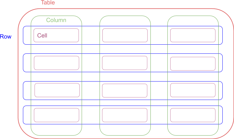
In SQL world Tables can represent relations between some entities (or objects) within a database system. Columns represent the entity attributes and Rows are tuples of data values that are mapped to these attributes. Schema dictates what data types the columns can hold, for example: text or numerical values, but in broader sense schema can also mean how tables are related (see Database schema). A cell is a value for a particualar row entry (intersection between a column and row). I will try to stick to this convention in the text below and in my future demo notebooks.

In my mind a SQL table looks something like a fancy burger:

When I first started working with databases the above definitions made my head spin. So let me try to clarify them a little bit.

I think of a SQL table as an abstract container that can hold a collection of objects. Say a table called fruits can hold fruit objects. Before we can create the table, we need to decide what kind of attributes, columns, we should store. For example, we can create a column name that will hold textual values such as “apple”, “pear” etc. and average_unit_weight holding numerical values such as 100.0, or 60.0 grams. Of course we can later come back and alter that. So name and average_unit_weight data types dictate our column schema and if you were to add textual value to numeric column you would get an error. Thus, SQL databases preserve data integrity after so you don’t get surprises after you did all that hard work to set it up.

Let’s now add two objects to the table with some example values: fruits(name="apple", average_unit_weight=55.7) and fruits(name="pear", average_unit_weight=64.7). If we were to select all the “name” values we would get two rows (tuples): ("apple") and ("pear").

Now if we were to inspect the table by selecting all values for two columns “name” and “average_unit_weight” we would get two rows: ("apple", 55.7) and ("pear", 64.7). We could keep repeating this for N number of columns.

In this way and if this makes sense so far, SQL table can have a specified number of columns and unspecified number of rows depending how much data we have added.

Many SQL database systems also allow us to add addional constains on cell data, for example we can specify for names to be unique to prevent duplication.

The most powerful feature of RDBMS is that we can make relations between objects in one table to objects in another table. Say we have created tables holding following objects with given columns:

customers(customer_id, name, delivery_address, account_number)

products(product_id, name, price, shipping_cost)

orders(product_id, customer_id, quantity, date_shipped, date_purchased)

stock(product_id, quantity)

Orders can give us information on what products have been sold so far because they can relate to products table by product_id. We can also check stock levels because we can form a relation to products table and deduce the quantity that has been shipped so far.

We can also make complex queries to unveil customer’s shopping habits to improve marketing etc.

Lastly, RDBMS can allow us to search for relevant information very efficiently because of their ability to build indices on specified table columns (or sets of columns). You can think of SQL database index to be a similar to a book’s contents table which can tell you the page number of relevant topic that you want to look up. Viewing the contents table first can protect your sanity from going through every page of the book. I will touch this topic in a future demo.

Project setup

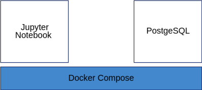
I have greated a project on Github, here. The PostgreSQL is set up to run inside Docker container and we will use Jupyter Notebook as a client, which also runs inside Docker container. Both SQL and Notebook services are orchestrated by Docker-Compose. The set up is simple as and can be visualised as:

Requirements

This project is meant to be run on Linux systems, Ubuntu in my case (sorry Windows you are too difficult).

I assume you have basic knowledge of Python, Makefiles, Linux Docker and Docker Compose.

I created a Makefile that should make it easier, I hope, to run and play with the project.

You should play with it as you wish, but I would recommend you to play the notebook’s code sections sequentially. You should also create your own tables and relations to explore PosgreSQL further.

To check all required components and optional components, pipenv and pyenv, for the project run in the project folder:

make check_system

This should give you similar output:

# System details
LSB Version:    core-9.20170808ubuntu1-noarch:security-9.20170808ubuntu1-noarch
Distributor ID: Ubuntu
Description:    Ubuntu 18.04 LTS
Release:        18.04
Codename:       bionic
# Docker components
Docker version 18.06.3-ce, build d7080c1
docker-compose version 1.23.2, build 1110ad01
# Pipenv version
pipenv, version 2018.11.26
# Pyenv version
pyenv 1.2.17-1-g89786b90

Running demo

To start docker containers run:

make run

You should access the notebook on

http://localhost:8888/?token=[TOKEN_VALUE]

The url with token should appear in your console output.

To stop the project either press ctrl+c or use:

make stop

The above command should also reset Docker volumes.

If you want to explore some database engine commands directly run:

make db_container_login

Once you are logged on the db, \? should give you information about commands beginning with \ and \h lists information about SQL commands.

For example, running \h CREATE TABLE should produce similar output (I truncated the output to first usage example):

demo-db=# \h CREATE TABLE
Command:     CREATE TABLE
Description: define a new table
Syntax:
CREATE [ [ GLOBAL | LOCAL ] { TEMPORARY | TEMP } | UNLOGGED ] TABLE [ IF NOT EXISTS ] table_name ( [
{ column_name data_type [ COLLATE collation ] [ column_constraint [ ... ] ]
    | table_constraint
    | LIKE source_table [ like_option ... ] }
    [, ... ]
] )
[ INHERITS ( parent_table [, ... ] ) ]
[ PARTITION BY { RANGE | LIST | HASH } ( { column_name | ( expression ) } [ COLLATE collation ] [ opclass ] [, ... ] ) ]
[ USING method ]
[ WITH ( storage_parameter [= value] [, ... ] ) | WITHOUT OIDS ]
[ ON COMMIT { PRESERVE ROWS | DELETE ROWS | DROP } ]
[ TABLESPACE tablespace_name ]

Alternatively you can connect to the PosgresSQL database using your favorite client with connection settings given in the Makefile.

Assuming you managed to navigate to Jupyter service and opened PostgreSQL Demo 1.ipynb notebook, you should see content similar to the one below (if not report issues in comments):

PostgreSQL Demo 1

In this demo we will explore:

- how to create a connection to PostgreSQL
- basic CRUD operations, mnemonic for:
    - Create tables
    - Read tables
    - Update tables
    - Delete tables
- table Joins

import os
import psycopg2
import sqlalchemy
import pprint as pp

Create a connection to PostgreSQL

To make a connection we use SQLAlchemy’s create_engine call to create a new engine instance through which we will make calls to our database application programming interface (DB API).

See the details on how SQLAlchemy interacts with DB API: SQLAlchemy engines

Note: we use postgresql to tells SQLAlchemy to specify DB type and psycopg2 noun explicity. pscopg2 is an adapter that let’s us make calls specifically to PostgreSQL.

# get settings from env variables that were passed around from makefile to docker-compose
SQL_PORT=os.environ['POSTGRES_PORT']
SQL_DB=os.environ['POSTGRES_DB']
SQL_USER=os.environ['POSTGRES_USER']
SQL_PASSWORD=os.environ['POSTGRES_PASSWORD']
SQL_SERVICE_NAME='postgres'

# create an engine that will allow us to communicate with PostgresSQL containerised server
engine = sqlalchemy.create_engine(f'postgresql+psycopg2://{SQL_USER}:{SQL_PASSWORD}@{SQL_SERVICE_NAME}/{SQL_DB}')

# just list our existing tablenames, on first run this should be empty, so check if that is the case
engine.table_names()

Python helpers

NOTE: I wanted to make these example as simple as possible. However, I used SQLAlchemy library to manage interaction with PostgreSQL server which might be slightly excessive. Nonetheless, I wanted to introduce it now so we can return to it in future demos when we begin writing more declarative code.

The following Python functions simplify our interaction with PostgreSQL:

# define helper functions that wrap our SQL statements

def execute_sql_statement(sql_statement):
    """Helper to execute sql statements like Inserts, Deletes, Updates that we don't
        need any feedback for this demo
    """
    with engine.connect() as connection:
        try:
            connection.execute(sql_statement)
        except Exception as e:
            print(e)

def get_header_rows(select_sql_statement):
    """Helper to execute select statements and bring back data
    """
    header = rows = None

    with engine.connect() as connection:
        ResultProxy = connection.execute(select_sql_statement)
        header = ResultProxy.keys()
        rows =  ResultProxy.fetchall()
    return header, rows

DROP & CREATE table

Let us create our first SQL table called countries to which we will add some data.

First we will want to make sure countries table does not exits so we will first run a SQL statement:

DROP TABLE IF EXISTS countries;

The DROP statement will instruct SQL server to find and delete countries table IF it EXISTS.

Now to create a new countries table we will be executing a statement:

CREATE TABLE countries (
    country_code char(2) PRIMARY KEY,
    currency_code char(3),
    country_name text UNIQUE
);

The above Schema defining a countries table instructs SQL server to create a column country_code that can accept a row value constrained to two characters and three characters for currency_code. text means that country_name can have any length, however, the UNIQUE constraint prevents duplicate entries (see documentation for more https://www.postgresql.org/docs/9.1/datatype-character.html)

PRIMARY KEY is a unique, non-null, row identifier and will be a lookup for that table. I will revisit primary keys in the next demo when we introduce a concept of SQL index.

NOTE: SQL statement formatting does not matter during execution but it still should be formatted for maximum readability. The SQL clauses do not need capitalisation, however, it is a convention intended improved readability.

These instructions can be executed in Python as follwing:

# create `countries` table
insert_countries_table = """
DROP TABLE IF EXISTS countries;

CREATE TABLE countries (
    country_code char(2) PRIMARY KEY,
    currency_code char(3),
    country_name text UNIQUE
);
"""
execute_sql_statement(insert_countries_table)

engine.table_names()

INSERT INTO table

Now given we have a table with specified schema, we can add few entries.

The following statement instructs SQL server to add 5 rows:

INSERT INTO countries
    (country_code, currency_code, country_name)
VALUES
    ('US', 'USD', 'United States'),
    ('GB', 'GBP', 'United Kindgodm'),
    ('FR', 'EUR', 'France'),
    ('NG', 'NGN', 'Nigeria'),
    ('AT','ATX','Atlantida');

# Lets create some entries into the countries table with the following SQL insert statment
# Note that we are conforming ourselves to the defined data schema
insert_countries_data = """
INSERT INTO countries
    (country_code, currency_code, country_name)
VALUES
    ('US', 'USD', 'United States'),
    ('GB', 'GBP', 'United Kindgodm'),
    ('FR', 'EUR', 'France'),
    ('NG', 'NGN', 'Nigeria'),
    ('AT','ATX','Atlantida');
"""
execute_sql_statement(insert_countries_data)

SELECT * FROM table

Now we would like to inspect if the data has been stored. We can Read all rows for all columns from the countries table by calling:

SELECT * FROM countries;

What the above statement says: “read all, denoted by *, rows from countries table”.

Note: usually when you have larger tables it is wise to select few columns and use a LIMIT statement if you just want to inspect the data. For example:

SELECT col1, col2, col7 FROM table_name LIMIT 20;

Let’s do this execute the above with Python and let’s see some results

# To view the Table's rows, we can execute following SQL query
select_countries = """
SELECT * FROM countries;
"""

country_header, country_rows =  get_header_rows(select_countries)

pp.pprint(country_header)
pp.pprint(country_rows)
pp.pprint("*"*50)
pp.pprint("Note: we extracted the header and the country rows into separate variables but in SQL these are mapped like below:")
pp.pprint("*"*50)
pp.pprint([dict(zip(country_header, row)) for row in country_rows])

Side Notes on SQLAlchemy Metadata, Table objects

There is an alternative method, and probably more Pythonic, to run sql statements using SQLAlchemy.

For example we can select all countries by using SQLAlchemy’s Table and Metadata objects like in the example below. This gives the same results.

You can read more in here: https://www.sqlalchemy.org/

metadata = sqlalchemy.MetaData()
countries = sqlalchemy.Table('countries', metadata, autoload=True, autoload_with=engine)

query = sqlalchemy.select([countries])

with engine.connect() as connection:

    ResultProxy = connection.execute(query)
    countries_results_2 = ResultProxy.fetchall()

countries_results_2

DELETE FROM table

We introduced a mistake and added Atlantida as country. Let’s remove the row by using DELETE clause and referencing its specific country_code by using WHERE statement:

DELETE
FROM countries
WHERE country_code = 'AT';

Then let’s use select to see the result:

delete_atlantida = """
DELETE
FROM countries
WHERE country_code = 'AT';
"""

execute_sql_statement(delete_atlantida)

select_countries = """
SELECT *
FROM countries;
"""

country_header, country_rows =  get_header_rows(select_countries)

print(country_header)
pp.pprint(country_rows)

ALTER table

Let’s also modify, sql speaking ALTER TABLE, a column currency_code. It doesn’t really belong in here so we want to remove it, DROP COLUMN. To do that we run:

ALTER TABLE countries DROP COLUMN IF EXISTS currency_code;

The statement will instruct SQL server to remove mapping between currency_code column and data rows.

delete_currency_col = "ALTER TABLE countries DROP COLUMN  IF EXISTS  currency_code;"

execute_sql_statement(delete_currency_col)


select_countries = """
SELECT *
FROM countries;
"""
country_header, country_rows =  get_header_rows(select_countries)

print(country_header)
pp.pprint(country_rows)

Adding and populating more tables - currency

Let’s add another table called currency with following schema and populate it with some data:

DROP TABLE IF EXISTS currency;

CREATE TABLE currency (
    currency_code char(3) PRIMARY KEY,
    country_code char(2) REFERENCES countries (country_code),
    currency_desc varchar(45)
);

Note that I used REFERENCES noun that tells SQL to lookup country_code in countries table.

add_currency_table = """
DROP TABLE IF EXISTS currency;

CREATE TABLE currency (
    currency_code char(3) PRIMARY KEY,
    country_code char(2) REFERENCES countries (country_code),
    currency_desc varchar(45)
);
"""

execute_sql_statement(add_currency_table)

insert_currency_data = """
INSERT INTO currency
    (currency_code, country_code, currency_desc)
VALUES
    ('USD', 'US', 'US Dollar'),
    ('GBP', 'GB', 'British Pound'),
    ('EUR', 'FR', 'Euro'),
    ('NGN', 'NG', 'Nigerian Naira');
"""

execute_sql_statement(insert_currency_data)

currency_header, currency_rows =  get_header_rows("SELECT * FROM currency;")

print(currency_header)
pp.pprint(currency_rows)

If we try to add new currency that that has got a defined country in REFERENCE table we get an error. Why is that? SQL server tries to maintian referential integrity i.e. if reference does not exist, throw an error rather than allow to incorrect data to be inserted

insert_currency_data = """
INSERT INTO currency
    (currency_code, country_code, currency_desc)
VALUES
    ('ATT', 'AT', 'Atlantida Lyra')
"""

execute_sql_statement(insert_currency_data)

We can still insert the data with Null reference which in some cases is not a ideal, but we can update the data at some later time.

insert_currency_data_2 = """
INSERT INTO currency
    (currency_code, country_code, currency_desc)
VALUES
    ('VEB', Null, 'Bolivar')
"""

execute_sql_statement(insert_currency_data_2)

currency_header, currency_rows =  get_header_rows("SELECT * FROM currency")

print(currency_header)
pp.pprint(currency_rows)

Table Joins

Sometimes we want to make a query and find some common information between tables. This is where SQL databases shine. The power of relational database systems comes from their ability to take two or more tables and combine them in some way to produce a single table.

There are several types of join (see Join_(SQL) ), inner join is one of the simplest examples. In set theory, inner join represents an intersection of two sets of objects that share some common data attributes in some way. Take this silly diagrammatic example where we have a set of blue and yellow cows, cows with yellow-blue patches belong to this intersection subset:

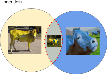
Let’s join currency and countries tables. To do this we use INNER JOIN clause and we use a ON countries.country_code = currency.country_code condition because it is a common column between the tables:

SELECT countries.*, currency_code
FROM countries INNER JOIN currency
ON countries.country_code = currency.country_code

The statement will select all columns from countries table and a currency_code from currency table and matches the condition.

This resulting table is what we originally started with. But now we have two independent tables which gives us more control and avoids too much duplication.

join_example_1 = """
SELECT countries.*, currency_code
FROM countries INNER JOIN currency
ON countries.country_code = currency.country_code
"""

join_ex1_header, join_ex1_rows =  get_header_rows(join_example_1)

print(join_ex1_header)
pp.pprint(join_ex1_rows)

Adding more tables - vendors, ecommerce_campaigns

Let us create even more tables. Make a note of the schema and various clauses like CHECK, SERIAL, DEFAULT and NOT NULL which you can read about more in the documentation.

create_vendors_table = """
DROP TABLE IF EXISTS vendors;
CREATE TABLE vendors (
vendor_id SERIAL PRIMARY KEY,
name varchar(255),
web_url text UNIQUE CHECK (web_url <> ''),
type char(7) CHECK (type in ('public', 'private') ) DEFAULT 'public',
country_code char(2) REFERENCES countries (country_code) NOT NULL,
operating_currency char(3) REFERENCES currency (currency_code) NOT NULL
)
"""
execute_sql_statement(create_vendors_table)

# Now check if we have 3 tables countries, currency, vendors
engine.table_names()

create_vendor_data = """
INSERT INTO vendors (name, web_url, type, country_code, operating_currency)
VALUES (
'Puppy world', 'https://puppy-world.eu', 'public', 'FR', 'EUR'
),
('Sporty socks', 'https://sporty-socks.co.uk', 'public', 'GB', 'GBP')
"""

execute_sql_statement(create_vendor_data)

# let's inspect vendor data
vendors_header, vendors_rows =  get_header_rows("SELECT * FROM vendors;")

print(vendors_header)
pp.pprint(vendors_rows)

# create campaign table
create_ecommerce_campaigns_table = """
DROP TABLE IF EXISTS ecommerce_campaigns;
CREATE TABLE ecommerce_campaigns (
    title varchar(255) CHECK (title <> ''),
    starts_at DATE NOT NULL,
    ends_at DATE CHECK (ends_at > starts_at),
    vendor_id int REFERENCES vendors (vendor_id)
)
"""

execute_sql_statement(create_ecommerce_campaigns_table)

# add campaign data
create_campaign_data = """
INSERT INTO ecommerce_campaigns (title, starts_at, ends_at, vendor_id)
VALUES
    ('Happy Puppy Ads', '2020-03-01', '2020-05-13', 1) ,
    ('New Soles Ads', '2020-01-01', '2020-01-31', 2),
    ('Trendy Spring Jackets Ads', '2020-03-20', '2020-04-28', Null)
"""

execute_sql_statement(create_campaign_data)

ecommerce__header, ecommerce_campaings_rows =  get_header_rows("SELECT * FROM ecommerce_campaigns;")

print(ecommerce__header)
pp.pprint(ecommerce_campaings_rows)

Outer Join and Aliases

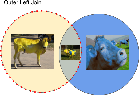
We want to list all ecommerce campaigns and check if any have an assigned online vendor or not. To do this we will use LEFT OUTER JOIN (you could use LEFT JOIN clause as well but let’s be explicit for the sake of this demo).

Diagramatically we can represent the left outer join as a set with objects from the left set of objects that also includes intersecting objects. Note that any objects that don’t match ON conditions will have Null values as a result.

We can also use aliases to make columns names more user friendly and tables names less verbose. To make use of an alias we can use AS clause. It is optional and we can omit it. I like keeping them in my queries but you might see queries without them.

SELECT
    ec.title AS "Campaign Name",
    ec.starts_at AS "Start Date",
    ec.ends_at AS "End Date",
    v.name AS "Signed Vendor"
FROM
    ecommerce_campaigns AS ec
LEFT OUTER JOIN  vendors AS v
ON
    ec.vendor_id = v.vendor_id

left_outer_join = """
SELECT
    ec.title AS "Campaign Name",
    ec.starts_at AS "Start Date",
    ec.ends_at AS "End Date",
    v.name AS "Signed Vendor"
FROM
    ecommerce_campaigns AS ec
LEFT OUTER JOIN  vendors AS v
ON
    ec.vendor_id = v.vendor_id
"""

left_join_header, left_join_results =  get_header_rows(left_outer_join)

print(left_join_header)
pp.pprint(left_join_results)

References

Image sources:

https://www.iflscience.com/plants-and-animals/millions-of-americans-think-chocolate-milk-comes-from-brown-cows/

https://www.afar.com/places/mysore-karnataka-mysore

https://www.waymarking.com/waymarks/WMQ7FV_Yellow_Cows_Bad_Imnau_Germany_BW